How do machines "learn"?
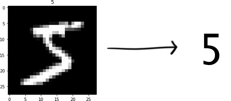
We’ll look at the classic problem of recognizing handwritten digits: the “Hello, world!” of machine learning. For humans with a fully developed visual cortex, this task is trivial. For a computer, this task is more complicated. We’ll solve this problem by building an artifical brain of sorts, a neural network. At its most basic level, a neural network is a function that takes an input and provides an output. The input to our function will be a 28x28 pixel grayscale image of a handwritten digit, and the output will be the digit represented in the image.
Perceptrons
Perceptrons are functions. They are the building blocks of neural networks and represent the indivudal neurons of the network. They take $n$ inputs, $x_0, x_1, x_2, …, x_n$, and produce one output: either $0$ or $1$.
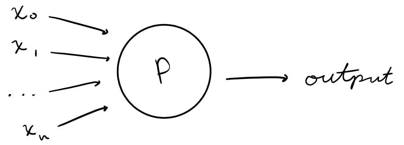
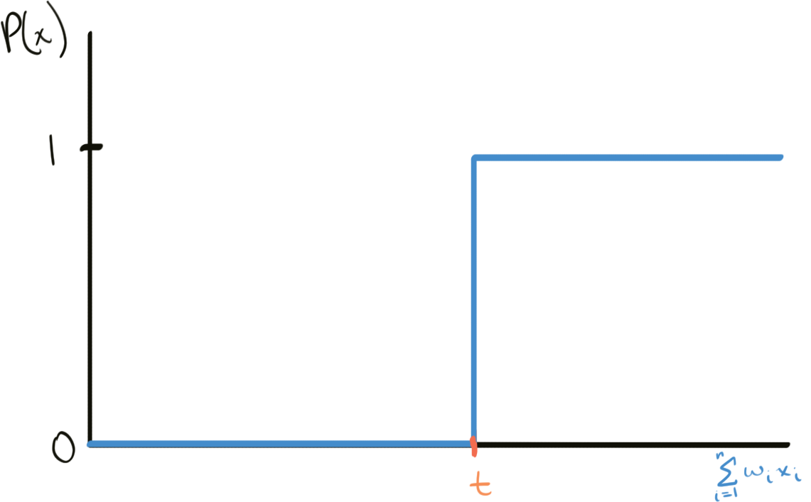
How is the output produced? Each perceptron has two types of real-number parameters: weights (one weight $w_n$ for each input $x_n$) and a threshold $t$. The output $P(x)$ of a perceptron is 1 if the weighted sum of the inputs $\sum_{i=0}^n w_a x_a$ is greater than or equal to $t$ and 0 if it is less than $t$.
Represented graphically:
and algebraically:
\[P(x) = \begin{cases} 1, & \text{if } \sum_{i=0}^n w_a x_a \ge t \\ 0, & \text{if } \sum_{i=0}^n w_a x_a \lt t \end{cases}\]Because there are many inputs $x$ and weights $w$, we can represent them as vectors where each component is one value of $x$ or $w$. Since the dot product between two vectors is defined as the weighted sum of its components, the function can be simplified to:
\[P(x) = \begin{cases} 1, & \text{if } \vec w \cdot \vec x \ge t \\ 0, & \text{if } \vec w \cdot \vec x \le t \end{cases}\]Moving $t$ to the other side of the equation will make it easier to manipulate later on. The threshold $t$ can also be expressed in terms of a bias $b$ where $t = -b$. We’ll use the bias from now on out of convention:
\[P(x) = \begin{cases} 1, & \text{if } \vec w \cdot \vec x + b \ge 0 \\ 0, & \text{if } \vec w \cdot \vec x + b \le 0 \end{cases}\]A weight $w_n$ represents the importance of the respective input $x_n$ to the output. A large weight $w_0$ means that $x_0$ has a large effect on the weighted sum and the output, and vice-versa. The bias is a threshold and represents how hard it is to get an output of 1. A large threshold will require large values of $x$ and large weights $w$. Initially, the weights and biases for each perceptron are chosen randomly. Later, we’ll see how calculus can be used to determine weights and biases that accurately represent the importance of inputs and the threshold for activation for a given problem.
Consider the parallels between how a human brain makes decisions. A variety of factors (inputs) are used to determine whether or not an action will be performed (output). For example, suppose you are deciding whether or not you should eat dinner tonight. Some inputs $\vec x$ might be how hungry you are $x_0$, what food you have at home $x_1$, and what the weather is outside $x_2$. Accurate weights will be high for the first two factors, $w_0$ and $w_1$, indicating that your hunger and the food you have at home play a large factor in your decision, and 0 for the last factor $w_2$, because the weather (shouldn’t) have any effect on your decision to eat dinner. Similarly, if the bias is high, it would indicate that you need to be very hungry (large value of $x_0$) and very hungry (large value of $x_1$) to choose to eat dinner (maybe you have high tolerance for hunger…)
Determining accurate values for the weights and biases involves tweaking the weights and biases and examining how it changes the output $P(x)$. If increasing the weights and/or biases moves the output closer to the correct answer, then the weights and/or biases need to increase, and vice-versa. In calculus terms, we need to find how the output changes with respect to a change in the weight and bias.
\[\Delta P = \sum_{i=0}^n \frac{\partial P}{\partial w_i}\Delta w_i + \frac{\partial P}{\partial b}\Delta b\]$\frac{\partial P}{\partial w}$ and $\frac{\partial P}{\partial b}$ are partial derivatives. They represent the same idea as a normal derivative; the change in $P$ with respect to the change in $w$ or $b$. The “partial” part indicates that F depends on multiple variables and that $w$ or $b$ is not the only variable that has an effect on $P$.
This requires differentiating the perceptron function with respect to $w$ and $b$. Unfortunately, this is not possible. Because it is a step function, the function is not differentiable at the threshold point $-b$. An infinitessimally small change in the weights at $-b$ can cause an infinitely large change in the output (from 0 to 1). At every other point the derivative is 0, making it impossible to know if the function is moving in the right or wrong direction. A modified perceptron is needed to solve this problem.

Sigmoid Neurons
What is really needed is a smooth perceptron function; one that is differentiable everywhere. We’ll still take the weighted sum as in the original perceptron, but instead of producing only a 0 or 1 if the weighted sum exceeds the bias $b$, the perceptron will produce any value between 0 and 1. This can be accomplished by passing the sum through an activation function. An activation function takes an input (in this case the weighted sum) and maps it to an output, which will be the output of the neuron. For this reason, the output of a neuron is called it’s activation. Knowing which activation function to use depends on the problem. We’ll use the logistic function $\sigma$ as our activation function:

Notice how the activation is bounded between 0 and 1. Very large sums produce activations very close to 1, while very small sums produce activations very close to 0.
There exists many other activation functions, such as the hyperbolic tan function or the ReLU function. The choice of activation function affects the efficiency of the network. Although not the most efficient, we chose the logistic function both for the sake of tutorial and because its derivatives are simple to compute.
Now we can represent the output of a single neuron as:
\[P(x) = \sigma(\vec w \cdot \vec x + b)\]The weighted sum plus bias is useful enough that we’ll define a variable for it. Let $z$ represent the weighted sum plus bias of a neuron:
\[\label{weightedSum} \begin{equation} z = \vec w \cdot \vec x + b \end{equation}\]Then the activation of a single neuron is:
\[\label{activation} \begin{equation} P(x) = \sigma(z) \end{equation}\]Connecting neurons together
A single neuron can’t make very complex decisions. Human brains have billions of neurons and it’s what allows us to think abstractly and make more complex decisions. Connecting individual neurons into a neural network enables a level of abstraction useful for solving more complex problems. “Connecting” individual neurons involves feeding the activation of one neuron into the input of another. How these connections are structured makes up the architecture of the neural network and affects how well a network can accurately model a problem. The choice of architecture therefore depends on the type of problem. A different architecture would be used for an image classification problem versus one of speech recognition. Although more effective architectures exist for image classification, we’ll use the most primitive type of architecture for simplicity: a feed-forward neural network.
A feed-forward neural network consists of $l$ layers, where each layer contains $k$ neurons. The inputs to a neuron in layer $l$ are the activations of every neuron in the previous layer $l-1$. Equivalently, the activation of a neuron in layer $l$ serve as one input to every neuron in layer $l+1$. The output of a layer $l$ can therefore be represented as a $k$-dimensional vector $a_l$, called the activation vector of layer $l$, where each component is the activation of one neuron in the layer. The choice of the number of layers and neurons per layer has an effect on the efficiency of the network. We’ll (somewhat arbitrarily) choose $l = 4$ layers.

The first layer $l = 0$, called the input layer, recieves the raw image data of the digit. Since there are $28 \cdot 28 = 784$ pixels in an image, this first layer will have $k = 784$ neurons. Each neuron will use the grayscale value (from 0 to 1) of one pixel as input (a grayscale value of 0 indicates the pixel is completely dark, while a value of 1 indicates the pixel is completely white).
The last layer $l = 3$, called the output layer, will output the network’s “guess” of the digit represented in the image. As there are 10 possible digits, the last layer will have $k = 10$ neurons. The corresponding output vector $a_3$ of this layer represents the how confidently the network thinks the given image is a specific digit. For example, an output vector of $a_3 = [0.40,0,0,0.80,0,0,0,0,0,0]$ means the network is $0.40 \cdot 100\% = 40\%$ confident that the given image is a 0, and $80\%$ confident that the image is a 3.
The two layers in between, $l = 1$ and $l = 2$ are called hidden layers whose purposes, among others, are to connect the input and output layers and abstract the raw inputs to meaningful outputs. Admittedly, calling the hidden layers “abstraction layers” is a bit of hand-waving, so it helps to intuitively think of them as offering extra weights and biases that can be tweaked to make the neural network more accurate.
Training
“Training” the network involves tweaking the weights and biases of each neuron so that the network can generate the correct output vector for any given image input. As mentioned before, we know we’re nudging the weights and biases in the right direction when the output vector $a$ gets closer to the answer. How do we know what the answer is? We use a dataset. A dataset contains input values tagged with the correct output value. The MNIST Dataset provides over 60000 of these training examples. With this, we can input an image into our network and compare the output vector with the tagged answer.
To quantify the closeness of the output vector to the correct answer, a cost function $C$ is defined:
\[\label{cost} \begin{equation} C(\vec w,B) = \frac{1}{2n}\sum_{j=1}^n ||y(\vec x_j)-\vec {a^L}||^2 \end{equation}\]This function is a quadratic cost function. For given weights $\vec w$ and biases $B$, $C(\vec w,B)$ gives the average error of the neural network over $n$ training examples.
$y(x_j)$ is the correct output vector derived from the tag for a training example $x_j$. $\vec {a^L}$ is the network’s output vector for a given training example $x_j$ and weights and biases $\vec w$ and $B$. A large value of $C(\vec w,B)$ indicates the network’s answers are not close to the correct answers, while a small value of $C(\vec w,B)$ indicates the network’s answers are close to the correct answers.
Representation of $\vec w$ and $B$
Remember that a network contains $l$ layers of neurons, and each layer can contain a different number of $j$ neurons. Because each neuron only has one bias associated with it, we can represent it with a matrix of biases $B$. Let $B^l_j$ represent the bias of the $jth$ neuron in the $lth$ layer. Then, the matrix $B$ is defined as:
\[B = \begin{bmatrix} b^0_0 & b^0_1 & b^0_2 & ... & b^0_j \\ b^1_0 & b^1_1 & b^1_2 & ... & b^1_j \\ b^2_0 & b^2_1 & b^2_2 & ... & b^2_j \\ & & ... & & \\ b^l_0 & b^l_1 & b^l_2 & ... & b^l_j \end{bmatrix}\]When representing weights, remember that each neuron does not only have one weight associated with it. Weights are associated with connections between neurons, not the neurons themselves. Any neuron in a feedforward network is connected to every neuron in the previous layer. Therefore, the $jth$ neuron in the $lth$ layer has $k$ weights associated with it, where $k$ is the number of neurons in the previous $(l-1)th$ layer. We can represent the weights associated with the connection between a layer $l$ and a layer $l-1$ as a matrix of weights $W^l$. Let $w_{j,k}$ represent the weight between the connection of the $jth$ neuron in the $lth$ layer and the $kth$ neuron in the $(l-1)th$ layer. Then, the matrix $W^l$ is defined as:
\[W^l = \begin{bmatrix} w_{0,0} & w_{0,1} & w_{0,2} & ... & w_{0,k} \\ w_{1,0} & w_{1,1} & w_{1,2} & ... & w_{1,k} \\ w_{2,0} & w_{2,1} & w_{2,2} & ... & w_{2,k} \\ & & ... & & \\ w_{j,0} & w_{j,1} & w_{j,2} & ... & w_{j,k} \end{bmatrix}\]We then need a weight matrix for every layer $l$ in the network. So, we define a vector $\vec w$ of weight matrices as:
\[\newcommand\colvec[1]{\begin{bmatrix}#1\end{bmatrix}} \vec w = \colvec{ W^0 \\ W^1 \\ W^2 \\ ... \\ W^l }\]for a network with $l$ layers.
Breaking down the cost function
\[||y(\vec x_j)-\vec {a^L}||\]Here, we are taking the magnitude of the difference between the correct vector $\vec y$ and the output vector $\vec N$ for one training example $x_j$. Notice that if these two are close in value, the magnitude of the difference will be small and so $C(\vec w,B)$ will be small. If they are far apart in value, the magnitude of the difference will be large and $C(\vec w,B)$ will be large.
\[||y(\vec {x_j})-\vec {a^L}||^2\]Squaring the magnitude of the difference is the namesake of the quadratic cost function. It penalizes answers that are very incorrect much worse than answers that are less incorrect. For example, if the magnitude of the difference is $5$ for a close, but incorrect answer, and $10$ for a very incorrect answer, the “cost” of the very incorrect answer is $\frac{10^2}{5^2} = \frac{100}{25} = 4$ times more expensive than the close answer if we square it. If we didn’t square it though, the very incorrect answer would only be $\frac{10}{5} = 2$ times more expensive.
\[\frac{1}{2n}\sum_{j=1}^n ||y(\vec x_j)-\vec a^L||^2\]Finally, we take the squared difference of each entry and average it over the entire training set by multiplying by $1/n$ (the extra $1/2$ coefficient will make differentiating this equation easier later on). We do this because we want the network to be able to generalize to any input image and not just one specific training example.
Notice that because of the squared difference, $C(\vec w, B)$ is always positive and that when the network gives the correct answer for every training example, $C(\vec w, B)$ is 0. The ultimate goal that will improve the network output then is to modify $\vec w$ and $B$ in a way that minimizes $C(\vec w,B)$.
Minimizing a multivariable function
Gradients
The gradient of a multivariable function $F$, denoted $\nabla F$, is a vector containing every partial derivative of F. Much like how a negative derivative indicates that a one-dimensional function is decreasing, the gradient can be used to describe the shape of a multivariable function at a certain point. For a function $F(x_0, x_1, …, x_n)$ with $n$ variables, its gradient is defined as:
\[\newcommand\colvec[1]{\begin{bmatrix}#1\end{bmatrix}} \nabla F = \colvec{ \frac{\partial F}{\partial x_0} \\ \frac{\partial F}{\partial x_1} \\ ... \\ \frac{\partial F}{\partial x_n} }\]Gradient descent
Minimizing a single-variable function is easy. Just find the point where the derivative is 0 to find the local extrema, and the smallest of these extrema is the global minimum. A function of 2 or 3 variables can be minimized in a similar way: finding the point where all the partial derivatives are equal to 0 and finding the smallest of the extrema. What do you do when a function contains thousands of variables in the form of weights and biases?
Gradient descent uses the gradient of a multivariable function $F$ to determine the direction of steepest descent at a point $P_0$. Once this direction is determined, a move is made in this direction from point $P_0$ to point $P_1$. This ensures that $F(P_1) < F(P_0)$ and that the difference $F(P_0) - F(P_1)$ is maximized. Then, the direction of steepest descent at point $P_1$ is found, and again a move is made from point $P_1$ to point $P_2$, etc. Repeating this process continually minimizes $F$ until eventually a minimum is attained and $\nabla F = 0$.
Visualizing gradient descent is easier in 3-dimensional space than in n-dimensional space, so we’ll consider the case of a two-dimensional function $G(x,y)$. It’s gradient is:
\[\nabla G = \colvec{ \frac{\partial G}{\partial x} \\ \frac{\partial G}{\partial y} }\]Consider a point $P = (x, y, G(x,y))$ on $G$. From $P$, what is the direction of steepest descent? In other words, if you were to stand at $P$ and move along a vector $\vec v$, what direction of $\vec v$ decreases $G$ the most? The gradient $\nabla G$ gives all the information needed. Notice that $\nabla G$ is itself a vector and so it has a direction. Because the components of $\nabla G$ are the rates of change of $G$ with respect to an infinitessimal movement in the $\hat x$ or $\hat y$ direction, the direction of the gradient $\nabla G$ by definition points in the direction of steepest ascent. Therefore, to get the direction of steepest descent, we simply reverse the direction of the gradient: $-\nabla G$. In conclusion, from a point $P$ on $F$, the direction of steepest descent is the direction of $-\nabla G$ at $P$.
For a one-dimensional function $H(x)$, multiplying its derivative $\frac{dH}{dx}$ at a certain point by a small change $\Delta x$ gives the approximate change in $H$.
\[\tag{G1} \label{deltaH} \begin{equation} \Delta H \approx \frac{dH}{dx} \cdot \Delta x \end{equation}\]$\Delta x$ needs to be small because $\frac{dH}{dx}$ is the instantaneous rate of change and might not stay constant along the entire function. Restricting $\Delta x$ to small values ensures that the derivative does not change too much, keeping the approximation of $\Delta H$ accurate.
Similarily, for a $2$-dimensional function $G(x,y)$, multiplying its gradient $\nabla G$ at a certain point by a small scaled $2$-dimensional vector $\eta\vec v$ gives the approximate change in $G$ in the direction of that vector.
\[\tag{G2} \label{deltaG} \begin{equation} \Delta G \approx \nabla G \cdot \eta\vec v \end{equation}\]A movement that minimizes $G$ is a movement where $\Delta G$ is as negative as possible. We can’t just choose an arbitrarily large negative scalar $\eta$, because $\eta\vec v$ needs to stay small for the same reason that $\Delta x$ needed to stay small in ($\ref{deltaH}$). Instead, we point $\vec v$ in the direction that decreases the value of $G$ the most. This is the direction of steepest descent, which was determined to be the direction of $-\nabla G$. From ($\ref{deltaG}$).
\[\tag{G3} \label{deltaGDescent} \begin{equation} \Delta G \approx \nabla G \cdot -\eta\nabla G = -\eta||\nabla G||^2 \end{equation}\]This shows that moving in the opposite direction of the gradient guarantees that $\Delta G < 0$. So, the movement made from point $P_n$ to point $P_{n+1}$ that minimizes $G$ is $-\eta\nabla G$. Repeating the following will minimize the function $G$:
\[\begin{equation} \begin{aligned} P_{n+1} &= P_n + \eta\vec v \\ &= P_n - \eta\nabla G \\ (P_{n+1,x}, P_{n+1,y}) &= (P_{n,x} - \eta\frac{\partial G}{\partial x}, P_{n,y} - \eta\frac{\partial G}{\partial y}) \end{aligned} \end{equation} \tag{G4} \label{minimizingStep}\]The choice of the value for the scalar $\eta$ is important. If $\eta$ is small, the size of each step is small and it will take many more iterations of gradient descent to reach a minimum. If $\eta$ is big, the size of each step will be bigger, but the approximation of $\Delta G$ in ($\ref{deltaG}$) will be less accurate and $P_n$ may never converge to a minimum.
Optional: Relating the change in G to the gradient through the directional derivative
From ($\ref{deltaG}$), if the scalar of $\vec v$ is infinitessimal, then $\nabla G$ multiplied by $\vec v’$, the scaled vector $\vec v$, gives the directional derivative $\nabla_{\vec v} G$. The directional derivative represents the instantaneous rate of change of $G$ in the direction of the vector $\vec v$.
\[\nabla_{\vec v} G = \nabla G \cdot \vec v\]The directional derivative in the direction of steepest descent is given by:
\[\begin{aligned} \nabla_{-\nabla G} G &= \nabla G \cdot -\nabla G \\ &= -\eta||\nabla G||^2 \end{aligned}\]As in ($\ref{deltaH}$) and ($\ref{deltaG}$), multiplying the directional derivative of a function by a small coefficient $\eta$ gives the approximate change in the function in the direction of the directional derivative:
\[\begin{aligned} \Delta G &\approx \nabla_{-\nabla G} G \cdot \eta \\ &= -\eta||\nabla G||^2 \end{aligned}\]This is equivalent to ($\ref{deltaGDescent}$).
Minimizing the cost function with gradient descent
Everything that was explored for the two dimensional function $G(x,y)$ extends to any \(n\)-dimensional function $F(x_0, x_1, …, x_n$). This includes the use of gradient descent for minimization. Since the cost function \(C(W,B)\) is an \(n\)-dimensional function where \(n\) is equal to the number of weights in all the matrices of \(\vec w\) plus the number of biases in the matrix \(B\), we can use gradient descent to minimize it. “Unpacking” the inputs of $C(\vec w, B)$ makes it more clear how $C$ is an n-dimensional function.
\[\begin{aligned} C(\vec w, B) & = C(W^0, W^1, ..., W^l, B) \\ & = C(w^0_{0,0}, w^0_{0,1}, ..., w^l_{j,k}, b^0_0, b^0_1, ..., b^l_j) \end{aligned}\]Exactly like how the point $P$ on a two-dimensional function $G(x,y)$ is defined as $(x,y,G(x,y))$, the point $P$ on an $n$-dimensional function $C(\vec w, B)$ is defined as:
\[P = (\vec w, B, C(\vec w, B))\]To move from a point $P_0$ on the cost function to a lower point $P_1$, we move in the opposite direction of the gradient by a scalar of $\eta$ as in $(\ref{minimizingStep})$:
\[\begin{aligned} P_{1} &= P_0 + \eta\vec v \\ &= P_0 - \eta\nabla C \\ (P_{1,\vec w}, P_{1,B}) &= (P_{0,\vec w} - \eta\frac{\partial C}{\partial \vec w}, P_{0,B} - \eta\frac{\partial C}{\partial B}) \end{aligned}\]Therefore, to minimize the cost function through gradient descent, we repeatedly apply the following operation to the vector of weight matrices $\vec w$ and the bias matrix $B$:
\[\begin{aligned} \vec w' & = \vec w - \eta\frac{\partial C}{\partial \vec w} \\ B' & = B - \eta\frac{\partial C}{\partial B} \end{aligned}\]To do this, we need to compute the cost gradient $\nabla C$ and choose a suitable value for $\eta$.
Computing the cost gradient $\nabla C$ using backpropagation
We want to compute the partial derivatives of $C$ with respect to $\vec w$ and $B$ so that we can form the gradient $\nabla C$.
\[\nabla C = \colvec{ \frac{\partial C}{\partial \vec w} \\ \frac{\partial C}{\partial B} }\]There are four fundamental equations of backpropgation (BP) that allow us to do this. We’ll derive each one of them.
Because the activations of each layer are influenced by the ones of every layer before it, we’ll need to differentiate one layer at a time. To do this, we’ll use a proxy variable that we can derive for any layer. Then, we only need to find one expression for the partial derivatives in terms of the proxy variable which can be used to determine the partial derivatives of every layer.
The proxy variable, $\delta^l$
Let $\delta^l$ be our proxy which represents the “error” of a layer $l$. What does the error of a layer mean? Think of it as a way to describe how much the cost function changed because of a layer $l$. Recall how each function feeds into the next:

Functions that are associated with the same layer are the same colour. Imagine the diagram as an assembly line. The initial raw materials are the pixels of the input image. They flow through each “worker” (layer), and each one applies some transformations to it until it becomes a final product (a digit classification) where it reaches quality assurance at the end of the line (the cost function). If we want to evaluate the error that a worker introduced into the assembly line, we should examine how the transformations that the worker applied changed the final product $C$. For the red worker, the “transformations” it applies are the weighted sum $z^L$, followed by the activation function $a^L$. Therefore, there is reason to believe that the error $\delta^L$ in the last red layer $L$ should be $\frac{\partial a^L}{\partial z^L}\frac{\partial C}{\partial a^L}$, which simplifies to $\frac{\partial C}{\partial z^L}$.
\[\tag{BP1} \label{lastError} \begin{equation} \delta^L = \frac{\partial C}{\partial z^L} \end{equation}\]What about the error in the layer before the last one? Returning to the assembly line analogy, if a worker introduces error early in the line, they’ll induce additional errors later in the line too. Later workers will mess up if they are forced to work on a malformed product! So, the error of the second last layer $l$ in the assembly line should be the transformations applied by that layer $l$, as well as the transformations applied by any future layers. Looking at the diagram, the second last blue layer applies the weighted sum $z^l$, followed by the activation function $a^l$. The transformation in the last red layer after that was determined above to be $\delta^L$. So, the error $\delta^l$ in the second last blue layer should be:
\[\delta^l = \frac{\partial a^l}{\partial z^l}\frac{\partial z^L}{\partial a^l}\delta^L\]Since $l$ is the second-last layer and $L$ is the last layer, then $L = l+1$. So, $\delta^l$ can be expressed in terms of the layer after it:
\[\tag{BP2} \label{anyError} \begin{equation} \delta^l = \frac{\partial a^l}{\partial z^l}\frac{\partial z^{l+1}}{\partial a^l}\delta^{l+1} \end{equation}\]By relating $\delta^l$ to $\delta^{l+1}$, we now have a way to determine the error of any layer by recursively applying the relation in $(\ref{anyError})$.
\[\delta^l \to \delta^{l-1} \to \delta^{l-2} \to ... \to \delta^1 \to \delta^0\]This technique is called “backpropagation” because we’re propagating the error backwards through the layers.
Differentiating the cost function with respect to the weights
Recall the cost function from $(\ref{cost})$:
\[C(\vec w,B) = \frac{1}{2n}\sum_{j=1}^n ||y(\vec x_j)-\vec {a^L}||^2\]Because $C$ is the average cost over all training examples, the final cost gradient $\nabla C$ will contain the average of the partial derivatives over all $n$ training examples. But, because we’ll compute the cost gradient one training example $x$ at a time anyway, instead of finding the average gradient over all training examples $\nabla C$, we’ll consider the gradient over just one fixed training example, $\nabla C_x$. (If we want to find the average gradient later, we can just sum $\nabla C_x$ and divide by $n$). This simplifies the cost function of one training example to:
\[C_x(\vec w,B) = \frac{1}{2}||y(\vec x_j)-\vec{a^l}||^2\]Notice that the only term in the cost function that depends on the weights is $\vec{a^l}$. So, in terms of $W^l$, $C$ is only a function of $\vec{a^l}$, which is a function of $\vec {z^l}$ (from $(\ref{activation})$) which is a function of $W^l$. This means, notationally by the chain rule (vector symbols are omitted for clarity):
\[\frac{\partial C}{\partial W^l} = \frac{\partial C}{\partial a^l}\frac{\partial a^l}{\partial z^l}\frac{\partial z^l}{\partial W^l}\]We’ll derive each of these partial derivatives (PDs) seperately and then multiply them together in the end to get $\frac{\partial C}{\partial W^l}$.
Deriving the cost w.r.t the last activations: $\frac{\partial C}{\partial a^l}$
Start with the simplified cost function:
\[\frac{\partial C}{\partial a^l} = \frac{\partial}{\partial a^l}\frac{1}{2}||y(\vec x_j)-a^l||^2\]Now it becomes apparent why the cost function contained the $\frac{1}{2}$ coefficient. By the power rule, this simplifies to:
\[\tag{PD1} \label{CwrtA} \begin{equation} \frac{\partial C}{\partial a^l} = ||y(\vec x_j)-a^l|| \end{equation}\]Deriving the last activations w.r.t the last weighted sum$\frac{\partial a^l}{\partial z^l}$
Start with the activation vector of a layer $l$ from $(\ref{activation})$:
\[\begin{aligned} \frac{\partial a^l}{\partial z^l} &= \frac{\partial}{\partial z^l}\sigma(z^l) \\ &= \sigma'(z^l) \end{aligned}\]Since:
\[\sigma(x) = \frac{1}{1+e^{-x}}\]Then by the quotient rule:
\[\sigma'(x) = - \frac{e^{-x}}{(1+e^{-x})^2}\]expressed in terms of $\sigma$:
\[\begin{aligned} \sigma'(x) &= -\frac{e^{-x}}{(1+e^{-x})^2} \\ &= \frac{1+e^{-x}}{(1+e^{-x})^2} - \frac{1}{(1+e^{-x})^2} \\ &= \frac{1}{1+e^{-x}} - \frac{1}{(1+e^{-x})^2} \\ &= \sigma(x)(1-\sigma(x)) \end{aligned}\]So,
\[\tag{PD2} \label{AwrtZ} \begin{equation} \frac{\partial a^l}{\partial z^l} = a^l(1-a^l) \end{equation}\]Deriving the last weighted sum w.r.t the weights $\frac{\partial z^l}{\partial W^l}$
This is the easiest of all of them. From the weighted sum $(\ref{weightedSum})$,
\[z^l_{j} = W^l_j \cdot a^{l-1} + B^l_j\]then
\[\tag{PD3} \label{ZwrtW} \begin{equation} \frac{\partial z^l}{\partial W^l} = a^{l-1} \end{equation}\]Putting it all together, using $(\ref{CwrtA}),(\ref{AwrtZ}),(\ref{ZwrtW})$, the partial derivative of the cost with respect to the weight matrix in the last layer is:
\[\frac{\partial C}{\partial W^l} = (y(\vec x_j)-a^l) \cdot a^l(1-a^l) \cdot a^{l-1}\]What about the partial derivative with respect to the weights in any layer? Now we’ll see why the proxy variable $\delta^L$ is useful. From $(\ref{lastError}), $(\ref{CwrtA}), and $(\ref{ZwrtW})$,
\[\begin{equation} \begin{aligned} \delta^L &= \frac{\partial C}{\partial z^L} \\ &= \frac{\partial C}{\partial a^L}\frac{\partial a^L}{\partial z^L} \\ &= (y(\vec x_j)-a^L)(a^L(1-a^L) \end{aligned} \end{equation} \tag{BP1'} \label{lastError2}\]and from $(\ref{anyError})$,
\[\begin{equation} \begin{aligned} \delta^l &= \frac{\partial a^l}{\partial z^l}\frac{\partial z^{l+1}}{\partial a^l}\delta^{l+1} \\ &= W^{l+1}(a^l(1-a^l)\delta^{l+1} \end{aligned} \end{equation} \tag{BP2'} \label{anyError2}\]So, we can succinctly express the partial derivative of the cost with respect to the weight matrix in any layer in terms of $\delta^l$:
\[\tag{BP3} \label{weightGradient} \begin{equation} \frac{\partial C}{\partial W^l} = \delta^l a^{l-1} \end{equation}\]Differentiating the cost function with respect to the biases
Luckily we’ve done most of the work for this already. We’ll apply the same logic we did for the weights and notice that the only term in the simplified cost function that depends on the biases is $\vec{a^l}$. So, in terms of $\vec {b^l}$, $C$ is only a function of $\vec{a^l}$, which is a function of $\vec {z^l}$ which is a function of $\vec {b^l}$. Again, by the chain rule,
\[\frac{\partial C}{\partial b^l} = \frac{\partial C}{\partial a^l}\frac{\partial a^l}{\partial z^l}\frac{\partial z^l}{\partial b^l}\]We can express this in terms of the error $\delta^l$:
\[\frac{\partial C}{\partial b^l} = \delta^l\frac{\partial z^l}{\partial b^l}\]Now we just have to derive for $\frac{\partial z^l}{\partial b^l}$.
Differentiating the last weighted sum w.r.t the biases $\frac{\partial z^l}{\partial b^l}$
Again, this is a simple one. From $(\ref{weightedSum})$,
\[z^l_{j} = W^l_j \cdot a^{l-1} + B^l_j\]then
\[\frac{\partial z^l}{\partial b^l} = 1\]Since $\frac{\partial z^l}{\partial b^l} = 1$, conveniently:
\[\tag{BP4} \label{biasGradient} \begin{equation} \frac{\partial C}{\partial b^l} = \delta^l \end{equation}\]Finally, we have a way to compute the cost gradient. The findings in this section can be summarised in just four equations.
The error of the last layer $(\ref{lastError2})$:
\[\delta^L = (y(\vec x_j)-a^L)(a^L(1-a^L)\]the error of any layer that is not the last one: $(\ref{anyError2})$
\[\delta^l = W^{l+1}a^l(1-a^l)\delta^{l+1}\]the partial derivative of the cost with respect to any weight $(\ref{weightGradient})$:
\[\frac{\partial C}{\partial W^l} = \delta^l a^{l-1}\]and the partial derivative of the cost with respect to any bias $(\ref{biasGradient})$:
\[\frac{\partial C}{\partial b^l} = \delta^l\]Stochastic Gradient Descent
Theoretically, taking the average cost gradient over all training examples $n$ gives the direction of steepest ascent. However, in practice, calculating all these partial derivatives is computationally expensive. Instead, we’ll approximate the average cost gradient by using a smaller mini-batch of training examples $m$ randomly selected (this is where “stochastic” in “stochastic gradient descent comes from” from $n$. Since our cost gradient isn’t exactly the average, the function might not step precisely in the direction of steepest descent. However, given enough iterations, the algorithm will still be able to minimize the function. We trade a bit of efficiency for a lot of speed.
So, instead of the cost function being:
\[C(\vec w,B) = \frac{1}{2n}\sum_{j=1}^n ||y(\vec x_j)-\vec{a^l}||^2\]it will be:
\[C(\vec w,B) = \frac{1}{2m}\sum_{j=1}^n ||y(\vec x_j)-\vec{a^l}||^2\]where $m < n$. Since these are effectively the same, our derivations for the cost gradient remain unchanged.
Implementing the neural network
Theoretically, we have everything we need to build a functioning neural network. In practice though, computational resources are expensive and time is limited. In this section, we’ll introduce the factors that need to be considered when moving from theory to practice.
Knowing when to stop gradient descent
If we let gradient descent run for an infinite amount of time, will the cost of our neural network eventually reach 0?
The answer is no.
The reason is that there is no guarantee that the minimum that gradient descent reaches is the absolute minimum. In fact, usually it’s not, simply because there is only one absolute minimum and many local minima. The minimum that gradient descent reaches depends on where our intial random weights and biases places us on the cost function. The global minimum will only be reached if we are placed on a portion of the graph that slopes downwards into the global minimum. So how do we know when to stop?
When the output of the cost function begins to converge at one value, it’s a good sign a local minimum was reached. Stopping training when the cost function begins to converge is important. Although you could squeeze out a bit more performance by letting the training continue to run, there runs a risk of the network learning data from the training examples that should just be noise. In essence, it would perform better for the specific training examples, but would be worse at generalizing to unknown problems (which is the important part). This is called overfitting. Stopping training before overfitting occurs is important for maintaining effective generalization of training examples.
Hyperparameters
Parameters for our neural network, such as the scalar $\eta$ used in gradient descent (called the learning rate), the mini-batch size m, the number of layers l, and the numbers of neurons in each of the layers are called hyperparameters They have a large effect on the efficiency of a network and their values can be the difference between a network that can learn to give correct answers and a network that spits out garbage. For this reason, optimizing for the right hyperparameters, called hyperparameter tuning is a large part of machine learning and is a growing area of study. The values for the hyperparameters given here were mostly found from trial and error, although there exists tools to help with hyperparameter tuning.
Code
Python is the language of choice for machine learning for good reason. Many of the linear algebra libraries used in machine learning, such as NumPy are written in C but can be interfaced with Python. This allows us to enjoy the abstraction and simplicity of Python with the speed of C.
Going over the code could be a seperate post entirely. Since this post is long enough, I’ll include the repository here, and maybe annotate another time.
github.com/davidtranhq/digit-recognizer
Additional resources: