Generating Images with Restricted Boltzmann Machines

The goal of unsupervised learning is to model the probability distribution $P_\text{data}(\bm x)$ of some type of data $\bm x$. Generating examples of $\bm x$ is hard because data in the real world is often extremely high-dimensional with complex distributions. If instead we represent $P_\text{data}(\bm x)$ with a simpler model $P_\text{model}(\bm x)$, we can generate new examples of $\bm x$ by sampling from $P_\text{model}(\bm x)$.

Complex probability distributions with multiple variables can be represented with a probabilistic graphical model. The probabilistic graphical model defines a graph $\mathcal{G}$ where each node corresponds to a variable and each edge corresponds to a possible dependence between the variables. The probability distribution can then be defined in terms of the nodes and the edges. In an undirected graphical model, if a node $X$ cannot be reached from a node $Y$, then $X$ and $Y$ are independent. If a node $X$ cannot be reached from a node $Y$ without passing through a node $Z$, then $X$ and $Y$ are conditionally independent given $Z$.

The restricted Boltzmann machine is an undirected graphical model with two layers: one layer of visible binary variables $\bm v$ and one layer of latent binary variables $\bm h$. The connections between the layers are given by a weight matrix $\bm W$, where $W_{i,j}$ represents the connection between $v_i$ and $h_j$. Intralayer connections are forbidden, forming a bipartite graph structure.

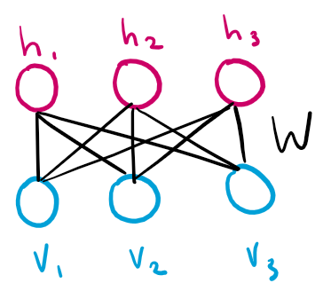
The goal is that the latent variables $\bm h$ will learn to represent the dependencies between the observed variables $\bm v$.

The model defines the joint probability distribution:

\[P(\bm v, \bm h) = \frac{1}{Z} \exp( -E(\bm v, \bm h))\]

where $E(\bm v, \bm h) = -\bm b^\top \bm v - \bm c^\top \bm h - \bm v^\top \bm W \bm h$ is the energy function. The parameters $\bm b$ and $\bm c$ are bias vectors for the visible and hidden variables, respectively. $Z$ is the partition function, the normalizing constant (with respect to $\bm v$ and $\bm h$) that ensures $P$ is a probability distribution by making $P$ sum to 1 over all $\bm v$ and $\bm h$.

\[Z = \sum_{\bm v} \sum_{\bm h} \exp(-E(\bm v, \bm h))\]

Note that the number of terms in $Z$ grows exponentially with respect to the number of dimensions of $\bm v$ and $\bm h$. So, if $\bm v$ or $\bm h$ are high-dimensional (as in most cases), $Z$ becomes intractable.

Gibbs Sampling

Because of the intractability of $Z$, exact samples can not be drawn from $P(\bm v, \bm h)$. Instead, a sample from $P(\bm v, \bm h)$ is approximated using Gibbs sampling.

In the most general form, Gibbs sampling is used to generate an $n$-dimensional sample $\bm x = \langle x_1, \dots, x_n \rangle$ from a joint probability distribution $P(\bm x)$. It is often used when the joint probability distirbution is difficult or impossible to sample from, but the conditional probability distributions are easy. The algorithm is as follows:

1. Initialize the initial sample $\bm x^{(0)}$ to some value (usually randomly or by some heuristic/algorithm).
2. Update the sample $\bm x^{(t)} \to \bm x^{(t + 1)}$ by sampling each $x_i^{(t+1)}$ individually from the conditional distribution $P(x_i^{(t+1)} \mid \mathbb X)$, where $\mathbb X = { x_1^{(t)}, \dots, x_n^{(t)} } \setminus { x_i^{(t)} }$ is the set of individual samples from the previous iteration, excluding the individual sample corresponding to $x_i^{(t+1)}$.
3. Perform $k$ iterations of the above step.

This process describes a Markov chain, where the state of the Markov chain is given by $P(\bm x^{(t)})$ and the transition operation $T$ is described in Step 2. When the Markov chain reaches a stationary distribution, $x^{(t)}$ becomes an exact sample from $P(\bm x)$. The number of iterations $k$ required for the Markov chain to converge to a stationary distribution is called the mixing time. Running the Markov chain until convergence is known as burning in the chain. Because $P(\bm x)$ is usually intractable, It is currently unknown how to determine the mixing time of an RBM’s Markov chain or to know when the Markov chain is mixed. So, most implementations halt after some constant number of iterations, say $k$. Although the sample is not exact, it is usually a good enough approximation.

Sampling Restricted Boltzmann Machines with Gibbs Sampling

A sample of $\bm v$ and $\bm h$ can be drawn from an RBM using Gibbs sampling. Because intralayer connections are prohibted in an RBM, an observed variable $v_i$ is conditioned only on $\bm h$. So, all $v_i \in \bm v$ are conditionally independent given $\bm h$. Therefore, rather than sampling each $v_i$ individually, the entire vector $\bm v$ can be sampled in parallel from $P(\bm v \mid \bm h)$ in Step 2 of the Gibbs sampling algorithm. Similarly, the entire vector $\bm h$ can be sampled in parallel from $P(\bm h \mid \bm v)$. Simultaneous sampling of conditionally independent variable while Gibbs sampling is called block Gibbs sampling.

The conditional probabilities for both are derived as follows:

\[\begin{aligned} P(\bm h = \bm 1 \mid \bm v) &= \frac{P(\bm v, \bm h = \bm 1)}{P(\bm v)} \\ &= \frac{P(\bm v, \bm h = \bm 1)}{P(\bm v, \bm h = \bm 1) + P(\bm v, \bm h = \bm 0)} \\ &= \frac{\exp(\bm b^\top \bm v + \bm c + \bm v^\top \bm W)}{\exp(\bm b^\top \bm v + \bm c + \bm v^\top \bm W) + \exp(\bm b^\top \bm v)} \\ &= \frac{\exp( \bm c + \bm v^\top \bm W)}{\exp(\bm c + \bm v^\top \bm W) + 1} \\ &= \sigma \left( \bm c + \bm v^\top \bm W \right) \end{aligned}\]

and symmetrically,

\[\begin{aligned} P(\bm v = \bm 1 \mid \bm h) &= \sigma \left( \bm b + \bm W \bm h\right). \end{aligned}\]

Training Restricted Boltzmann Machines with Maximum Likelihood

RBMs can be trained using maximum likelihood. Let $\bm x$ be the vector of variables in the model (including both observable variables and latent variables $\bm v$ and $\bm h$) and $\bm \theta$ the vector of parameters. Maximum likelihood is achieved using gradient ascent of the log-probability of the variables $\bm x$ with respect to the parameters $\bm \theta$. This gradient ascent requires computing the following gradient:

\[\nabla_{\bm \theta} \log P(\bm x; \bm \theta) = \nabla_{\bm \theta} \log \tilde P(\bm x; \bm \theta) - \nabla_{\bm \theta} \log Z\]

where $\tilde P(\bm x) = \exp(-E(\bm v, \bm h))$ is the unnormalized probability distribution. The positive and negative terms of this decomposition are called the positive and negative phases of learning, respectively.

The partial derivatives for the positive phase are given by:

\[\begin{aligned} \frac{\partial}{\partial \bm W}\left( -E(\bm v, \bm h)\right) &= \bm v \bm h^\top \\ \frac{\partial}{\partial \bm b}(-E(\bm v, \bm h)) &= \bm v \\ \frac{\partial}{\partial \bm h}(-E(\bm v, \bm h)) &= \bm h \end{aligned}\]

The partial derivatives for the negative phase are more difficult because of the intractability of $Z$. Instead, we work around $Z$ using the following identity:

\[\begin{aligned} \nabla_{\bm \theta} \log Z &= \frac{\nabla_{\bm \theta} Z}{Z} \\ &= \frac{1}{Z} \nabla_{\bm \theta}\sum_{\bm x} \tilde P(\bm x) \\ &= \frac{1}{Z} \sum_{\bm x} \nabla_{\bm \theta} \exp\left( \log\tilde P(\bm x)\right) \\ &= \frac{1}{Z} \sum_{\bm x} \exp\left( \log\tilde P(\bm x)\right) \nabla_{\bm \theta} \log\tilde P(\bm x) \\ &= \frac{1}{Z} \sum_{\bm x} \tilde P(\bm x) \nabla_{\bm \theta} \log\tilde P(\bm x) \\ &= \sum_{\bm x} P(\bm x) \nabla_{\bm \theta} \log\tilde P(\bm x) \\ &= \mathbb E_{\bm x \sim P}[\nabla_{\bm \theta}\log \tilde P(\bm x)] \end{aligned}\]

Note that the introduction of $\tilde P(\bm x) = \exp\left(\log \tilde P(\bm x)\right)$ is valid since $\tilde P(\bm x) > 0$.

Therefore, both the positive phase and negative phase involve computing $\nabla_{\bm \theta} \log \tilde P(\bm x)$. But, the positive phase samples $\bm x$ from the data, that is, $\bm v$ is sampled from the data $P_\text{data}(\bm v)$, and $\bm h$ is sampled from the model $P_\text{model}(\bm h \mid \bm v)$ given $\bm v$. The negative phase instead samples $\bm x$ from the model, that is, both $\bm v$ and $\bm h$ are sampled from $P_\text{model}(\bm v, \bm h)$ using Gibbs sampling.

Persistent Contrastive Divergence

Sampling $\bm v$ and $\bm h$ from $P(\bm v, \bm h)$ for the negative phase in maximum likelihood learning requires Gibbs sampling, which means burning in a new set of Markov chains at every gradient step. We can improve computational speed by using the assumption that the distribution defined by the model does not change too much between single gradient steps. Therefore, we can initialize each chain with the state of the chain from the previous gradient step to improve mixing time.

Note that this assumption requires that the learning rate be much smaller than if we initialized the Markov chains randomly. If the learning rate is too large, the model distribution will move faster than the Markov chains can mix.

Application

Treating Probabilities as Expectations

When computing the conditional posterior $P(\bm h \mid \bm v)$, it is common to take the probabilities of $\bm v$ as the values of $\bm v$ rather than sampling from the probabilities of $\bm v$ to reduce sampling noise. The theoretical justification is that since $\bm v$ is sampled from a Bernoulli distribution, using the probabilities of $\bm v$ is equivalent to taking the values of $\bm v$ to be the expectation of $\bm v$.

Note that when computing $P(\bm v \mid \bm h)$, it is important that $\bm h$ represents the binary values of the hidden units sampled from their probabilties and not the probabilities themselves. This acts as a regularizer, as it prevents the hidden units from communicating real-values to the visible units during reconstruction (Hinton, 2010).

Results

The RBM was implemented in PyTorch. It was trained on the MNIST dataset, with 50,000 samples used for training, 10,000 samples used for validation, and 10,000 samples used for testing. Each mini-batch comprised of 50 examples. The model was trained using persistent contrastive divergence with momentum and $L_2$ weight decay. The learning rate was decayed linearly from an initial value to zero over the course of training.

See https://github.com/davidtranhq/pytorch-rbm for the implementation. The parameter and hyperparameters for the below model can be found in the repository.

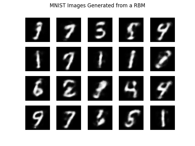
The following images were generated after 10 full steps of Gibbs sampling, initialized from random Markov chains. The images show the probabilities of the visible units.

The following images are reconstructions generated after 1 full step of Gibbs sampling, initialized from examples from the MNIST test set. Again, the probabilities of the visible units are shown.

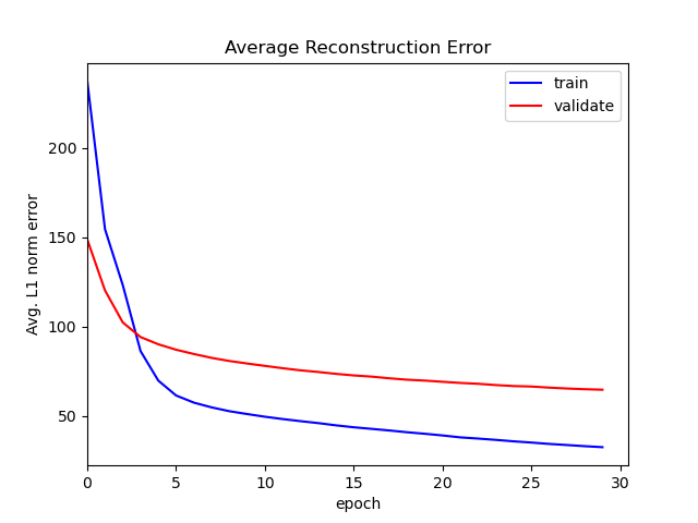
When training on the dataset, the input images are binarized with a threshold of 127. The reconstruction error is computed using the $L_1$ difference between the binary input and the binary reconstructions (sampled from $\bm v$).

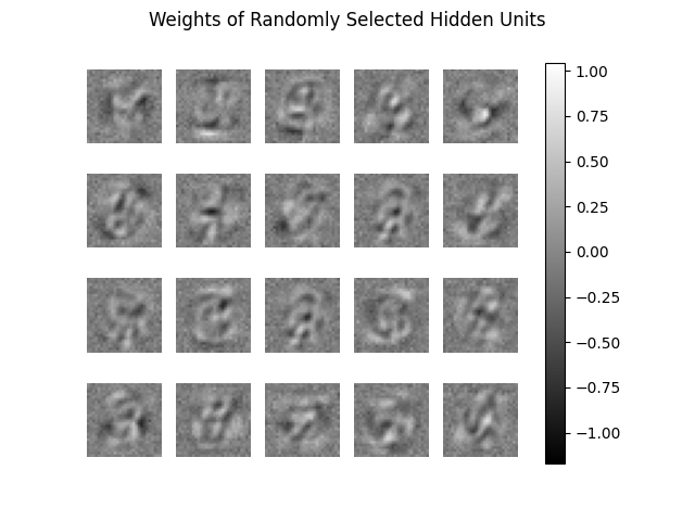
The weights of randomly selected hidden units are pictured below. Since each hidden unit is connected to the 28 x 28 = 784 visible units, each 28 x 28 image represents the weight between one hidden unit and all of the visible units.