Non-Uniform Random Number Generation

Most programming languages offer random number generators that can only generate uniformly-distributed random numbers. How can we use these to generate random numbers according to any distribution?

Let $U$ be a random variable with uniform distribution. We want to generate a random number $X = x$ from some distribution described by a probability density function $f(X)$. To generate $x$ using only $U$, we need to find a transformation $T$ such that $T(U) = X$.

Intuitively, we want $T(U)$ to map to high-probability values of $X$ more often than low-probability values of $X$. So, since $U$ is uniformly-distributed, a good transformation $T$ will concentrate larger regions of the domain of $U$ into the smaller regions of $X$ with high-probability density, thus increasing the chance of randomly picking some $u$ that maps to a high-probability valued $x$. One function that does this well is the inverse cumulative distribution function (also called the quantile function).

Inverse Cumulative Distribution Function

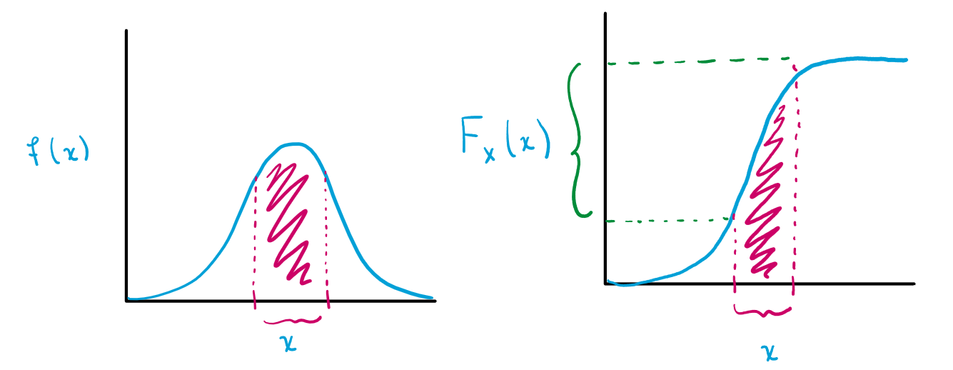
First, recall that the cumulative distribution function $F_X(x)$ for some random variable $X$ is defined as

\[F_X(x) = P(X \leq x)\]

where $P(X \leq x)$ is the probability that $X$ takes on a value less than or equal to $x$. We can compute this from the probability density function $f(X)$ as follows:

\[P(X \leq x) = \int_{-\infty}^x f(t) dt.\]

Notice how the cumulative distribution function increases most rapidly (covers many values of $F_X(x)$) when $f(x)$ is large:

Consequently, the inverse will map many values of $F_X(x)$ to the values of $x = F^{-1}_X(y)$ when $f(x)$ is large:

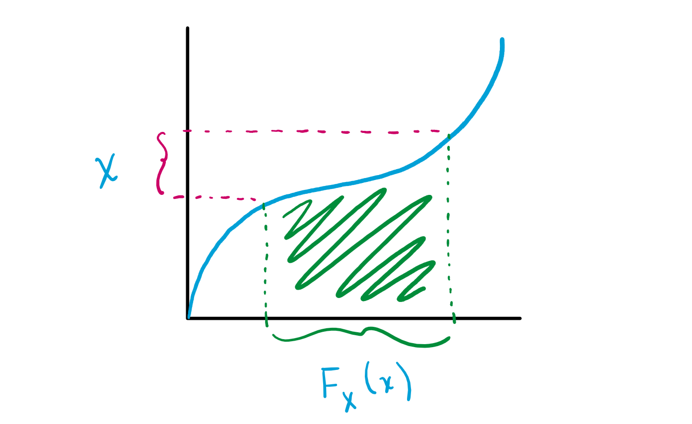
Thus, the inverse cumulative distribution function is intuitively a good choice of $T$ because it maps large regions of its domain to the smaller regions of $X$ where $f(X)$ is largest.

We can formalize this intution with the following theorem:

Theorem: Let $U$ be a standard uniformly-distributed random variable and let $F$ be a cumulative distribution function with inverse $F^{-1}$. Then, the cumulative distribution function of the random variable

\[X = F^{-1}(U)\]

is $F$.

Proof: From the definition of $F^{-1}(U)$,

\[\begin{aligned} F^{-1}(U) &= P(F^{-1}(U) \leq x) \\ &= P(U \leq F(x)) \\ &= F(x). \end{aligned}\]

since the cumulative distribution function $F_A$ of any standard uniformly-distributed random variable $A$ is $F_A(a) = P(A \leq a) = a$.

Example: Generating Random Points in a Circle

Let there be a circle centered at the origin with radius $R$. The task is to generate random points uniformly within the circle given only a uniformly-distributed random number generator $U(a, b)$.

A Naive Solution

An initial approach could be to generate random points in polar coordinates using a radius $r \sim U(0, R)$ and an angle $\theta \sim U(0, 2\pi)$. The probability of landing in a ring with an inner radius of $r_1$ and an outer radius of $r_2$ inside a circle of radius $R$ would be

that is, the area of the ring divided by the total area of the circle.

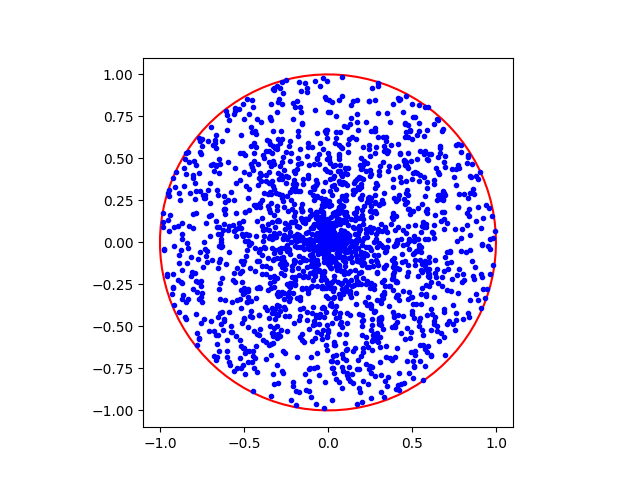
Unfortunately, this results in an overrepresentation of points nearer to the origin. The non-uniformity is because the relationship between a circle’s radius and its area is not linear but quadratic (since $A = \pi r^2$). Uniform sampling of the length of the radius thus does not result in uniform sampling of the regions in the circle. We can show this by comparing the area of the regions in the first half of the radius versus the second half:

\[A(r_1, r_2) = \pi r_2 ^2 - \pi r_1^2\]

where $r_1$ is the inner radius and $r_2$ is the outer radius, so

\[A\left(0, \frac{R}{2}\right) = \frac{1}{4}\pi R^2\] \[A\left(\frac{R}{2}, R\right) = \frac{3}{4}\pi R^2.\]

The area of the region in the first half of the radius is smaller. If we were to uniformly distribute the points by their radius, the region enclosed in the first half of the radius would have a much higher concentration of points as shown below:

A Uniform Solution

Instead, we can take advantage of the theorem from above. The cumulative distribution function $F(r)$, or the probability of landing within a circle of radius $r$ out of radius $R$, is given by

\[F(r) = p(r' \leq r) =\frac{\pi r^2}{\pi R^2} = \left(\frac{r}{R} \right)^2\]

so the inverse $F^{-1}(u)$ is

\[F^{-1}(u) = R\sqrt{u}\]

Note that the probability density function $f(r) = \frac{d F}{d r}(r) = 2\pi r$.

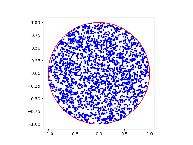
Then, by the theorem above, we can sample $r$ from the desired distribution defined by $f(r)$ by sampling $r \sim F^{-1}(U) = R\sqrt{U}$, where $U$ is a uniformly-distributed random variable between 0 and $R$.

Observe how the points are now uniformly distributed across the entire circle.

The code for generating both examples is given below.

import numpy as np
import matplotlib.pyplot as plt

def init_plot():
    _, ax = plt.subplots(1)
    ax.set_aspect(1)
    return ax

def draw_circle(ax, r=1.0):
    # generate contour points from polar coordinates
    theta = np.linspace(0, 2 * np.pi, 100)
    x = r * np.cos(theta)
    y = r * np.sin(theta)

    ax.plot(x, y, 'r')

def naive_points(ax):
    """Generate points by uniformly sampling (r,theta)."""
    num_pts = 2000

    r = np.random.rand(num_pts) # [0, 1]
    theta = np.random.rand(num_pts) * 2 * np.pi # [0, 2pi]

    x = r * np.cos(theta)
    y = r * np.sin(theta)

    ax.plot(x, y, 'b.')

def uniform_points(ax):
    """Generate points by uniformly sampling from the inverse cumulative."""
    num_pts = 2000

    u = np.random.rand(num_pts)
    r = np.sqrt(u) # u from U(0, 1)
    theta = np.random.rand(num_pts) * 2 * np.pi # [0, 2pi]

    x = r * np.cos(theta)
    y = r * np.sin(theta)

    ax.plot(x, y, 'b.')

# generate the naive plot
ax_naive = init_plot()
draw_circle(ax_naive)
naive_points(ax_naive)
plt.show()

# generate the true uniform plot
ax_uniform = init_plot()
draw_circle(ax_uniform)
uniform_points(ax_uniform)
plt.show()